使用keras實現(xiàn)CNN,直接上代碼:
from keras.datasets import mnist
from keras.models import Sequential
from keras.layers import Dense, Dropout, Activation, Flatten
from keras.layers import Convolution2D, MaxPooling2D
from keras.utils import np_utils
from keras import backend as K

class LossHistory(keras.callbacks.Callback):
    def on_train_begin(self, logs={}):
        self.losses = {'batch':[], 'epoch':[]}
        self.accuracy = {'batch':[], 'epoch':[]}
        self.val_loss = {'batch':[], 'epoch':[]}
        self.val_acc = {'batch':[], 'epoch':[]}

    def on_batch_end(self, batch, logs={}):
        self.losses['batch'].append(logs.get('loss'))
        self.accuracy['batch'].append(logs.get('acc'))
        self.val_loss['batch'].append(logs.get('val_loss'))
        self.val_acc['batch'].append(logs.get('val_acc'))

    def on_epoch_end(self, batch, logs={}):
        self.losses['epoch'].append(logs.get('loss'))
        self.accuracy['epoch'].append(logs.get('acc'))
        self.val_loss['epoch'].append(logs.get('val_loss'))
        self.val_acc['epoch'].append(logs.get('val_acc'))

    def loss_plot(self, loss_type):
        iters = range(len(self.losses[loss_type]))
        plt.figure()
        # acc
        plt.plot(iters, self.accuracy[loss_type], 'r', label='train acc')
        # loss
        plt.plot(iters, self.losses[loss_type], 'g', label='train loss')
        if loss_type == 'epoch':
            # val_acc
            plt.plot(iters, self.val_acc[loss_type], 'b', label='val acc')
            # val_loss
            plt.plot(iters, self.val_loss[loss_type], 'k', label='val loss')
        plt.grid(True)
        plt.xlabel(loss_type)
        plt.ylabel('acc-loss')
        plt.legend(loc="upper right")
        plt.show()

history = LossHistory()

batch_size = 128
nb_classes = 10
nb_epoch = 20
img_rows, img_cols = 28, 28
nb_filters = 32
pool_size = (2,2)
kernel_size = (3,3)
(X_train, y_train), (X_test, y_test) = mnist.load_data()
X_train = X_train.reshape(X_train.shape[0], img_rows, img_cols, 1)
X_test = X_test.reshape(X_test.shape[0], img_rows, img_cols, 1)
input_shape = (img_rows, img_cols, 1)

X_train = X_train.astype('float32')
X_test = X_test.astype('float32')
X_train /= 255
X_test /= 255
print('X_train shape:', X_train.shape)
print(X_train.shape[0], 'train samples')
print(X_test.shape[0], 'test samples')

Y_train = np_utils.to_categorical(y_train, nb_classes)
Y_test = np_utils.to_categorical(y_test, nb_classes)

model3 = Sequential()

model3.add(Convolution2D(nb_filters, kernel_size[0] ,kernel_size[1],
                        border_mode='valid',
                        input_shape=input_shape))
model3.add(Activation('relu'))

model3.add(Convolution2D(nb_filters, kernel_size[0], kernel_size[1]))
model3.add(Activation('relu'))

model3.add(MaxPooling2D(pool_size=pool_size))
model3.add(Dropout(0.25))

model3.add(Flatten())

model3.add(Dense(128))
model3.add(Activation('relu'))
model3.add(Dropout(0.5))

model3.add(Dense(nb_classes))
model3.add(Activation('softmax'))

model3.summary()

model3.compile(loss='categorical_crossentropy',
              optimizer='adadelta',
              metrics=['accuracy'])

model3.fit(X_train, Y_train, batch_size=batch_size, epochs=nb_epoch,
          verbose=1, validation_data=(X_test, Y_test),callbacks=[history])

score = model3.evaluate(X_test, Y_test, verbose=0)
print('Test score:', score[0])
print('Test accuracy:', score[1])

#acc-loss
history.loss_plot('epoch')
補充:使用keras全連接網(wǎng)絡訓練mnist手寫數(shù)字識別并輸出可視化訓練過程以及預測結果
前言
mnist 數(shù)字識別問題的可以直接使用全連接實現(xiàn)但是效果并不像CNN卷積神經(jīng)網(wǎng)絡好�����。Keras是目前最為廣泛的深度學習工具之一�,底層可以支持Tensorflow、MXNet�����、CNTK�、Theano
準備工作
TensorFlow版本:1.13.1
Keras版本:2.1.6
Numpy版本:1.18.0
matplotlib版本:2.2.2
導入所需的庫
from keras.layers import Dense,Flatten,Dropout
from keras.datasets import mnist
from keras import Sequential
import matplotlib.pyplot as plt
import numpy as np
Dense輸入層作為全連接,F(xiàn)latten用于全連接扁平化操作(也就是將二維打成一維)�,Dropout避免過擬合��。使用datasets中的mnist的數(shù)據(jù)集,Sequential用于構建模型�����,plt為可視化���,np用于處理數(shù)據(jù)��。
劃分數(shù)據(jù)集
# 訓練集 訓練集標簽 測試集 測試集標簽
(train_image,train_label),(test_image,test_label) = mnist.load_data()
print('shape:',train_image.shape) #查看訓練集的shape
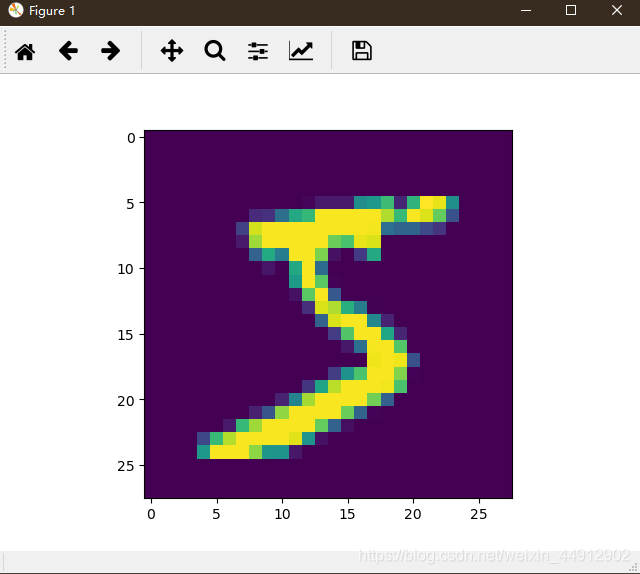
plt.imshow(train_image[0]) #查看第一張圖片
print('label:',train_label[0]) #查看第一張圖片對應的標簽
plt.show()
輸出shape以及標簽label結果:
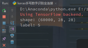
查看mnist數(shù)據(jù)集中第一張圖片:
數(shù)據(jù)歸一化
train_image = train_image.astype('float32')
test_image = test_image.astype('float32')
train_image /= 255.0
test_image /= 255.0
將數(shù)據(jù)歸一化��,以便于訓練的時候更快的收斂�����。
模型構建
#初始化模型(模型的優(yōu)化 ---> 增大網(wǎng)絡容量����,直到過擬合)
model = Sequential()
model.add(Flatten(input_shape=(28,28))) #將二維扁平化為一維(60000,28,28)---> (60000,28*28)輸入28*28個神經(jīng)元
model.add(Dropout(0.1))
model.add(Dense(1024,activation='relu')) #全連接層 輸出64個神經(jīng)元 ,kernel_regularizer=l2(0.0003)
model.add(Dropout(0.1))
model.add(Dense(512,activation='relu')) #全連接層
model.add(Dropout(0.1))
model.add(Dense(256,activation='relu')) #全連接層
model.add(Dropout(0.1))
model.add(Dense(10,activation='softmax')) #輸出層�,10個類別,用softmax分類
每層使用一次Dropout防止過擬合�����,激活函數(shù)使用relu�,最后一層Dense神經(jīng)元設置為10���,使用softmax作為激活函數(shù),因為只有0-9個數(shù)字��。如果是二分類問題就使用sigmod函數(shù)來處理�。
編譯模型
#編譯模型
model.compile(
    optimizer='adam',      #優(yōu)化器使用默認adam
    loss='sparse_categorical_crossentropy', #損失函數(shù)使用sparse_categorical_crossentropy
    metrics=['acc']       #評價指標
)
sparse_categorical_crossentropy與categorical_crossentropy的區(qū)別:
sparse_categorical_crossentropy要求target為非One-hot編碼,函數(shù)內(nèi)部進行One-hot編碼實現(xiàn)�。
categorical_crossentropy要求target為One-hot編碼。
One-hot格式如: [0,0,0,0,0,1,0,0,0,0] = 5
訓練模型
#訓練模型
history = model.fit(
    x=train_image,                          #訓練的圖片
    y=train_label,                          #訓練的標簽
    epochs=10,                              #迭代10次
    batch_size=512,                         #劃分批次
    validation_data=(test_image,test_label) #驗證集
)
迭代10次后的結果:

繪制loss���、acc圖
#繪制loss acc圖
plt.figure()
plt.plot(history.history['acc'],label='training acc')
plt.plot(history.history['val_acc'],label='val acc')
plt.title('model acc')
plt.ylabel('acc')
plt.xlabel('epoch')
plt.legend(loc='lower right')
plt.figure()
plt.plot(history.history['loss'],label='training loss')
plt.plot(history.history['val_loss'],label='val loss')
plt.title('model loss')
plt.ylabel('loss')
plt.xlabel('epoch')
plt.legend(loc='upper right')
plt.show()
繪制出的loss變化圖:

繪制出的acc變化圖:

預測結果
print("前十個圖片對應的標簽: ",test_label[:10]) #前十個圖片對應的標簽
print("取前十張圖片測試集預測:",np.argmax(model.predict(test_image[:10]),axis=1)) #取前十張圖片測試集預測
打印的結果:

可看到在第9個數(shù)字預測錯了���,標簽為5的,預測成了6���,為了避免這種問題可以適當?shù)募由罹W(wǎng)絡結構��,或使用CNN模型���。
保存模型
model.save('./mnist_model.h5')
完整代碼
from keras.layers import Dense,Flatten,Dropout
from keras.datasets import mnist
from keras import Sequential
import matplotlib.pyplot as plt
import numpy as np
# 訓練集 訓練集標簽 測試集 測試集標簽
(train_image,train_label),(test_image,test_label) = mnist.load_data()
# print('shape:',train_image.shape) #查看訓練集的shape
# plt.imshow(train_image[0]) #查看第一張圖片
# print('label:',train_label[0]) #查看第一張圖片對應的標簽
# plt.show()
#歸一化(收斂)
train_image = train_image.astype('float32')
test_image = test_image.astype('float32')
train_image /= 255.0
test_image /= 255.0
#初始化模型(模型的優(yōu)化 ---> 增大網(wǎng)絡容量,直到過擬合)
model = Sequential()
model.add(Flatten(input_shape=(28,28))) #將二維扁平化為一維(60000,28,28)---> (60000,28*28)輸入28*28個神經(jīng)元
model.add(Dropout(0.1))
model.add(Dense(1024,activation='relu')) #全連接層 輸出64個神經(jīng)元 ,kernel_regularizer=l2(0.0003)
model.add(Dropout(0.1))
model.add(Dense(512,activation='relu')) #全連接層
model.add(Dropout(0.1))
model.add(Dense(256,activation='relu')) #全連接層
model.add(Dropout(0.1))
model.add(Dense(10,activation='softmax')) #輸出層�,10個類別,用softmax分類
#編譯模型
model.compile(
optimizer='adam',
loss='sparse_categorical_crossentropy',
metrics=['acc']
)
#訓練模型
history = model.fit(
x=train_image, #訓練的圖片
y=train_label, #訓練的標簽
epochs=10, #迭代10次
batch_size=512, #劃分批次
validation_data=(test_image,test_label) #驗證集
)
#繪制loss acc 圖
plt.figure()
plt.plot(history.history['acc'],label='training acc')
plt.plot(history.history['val_acc'],label='val acc')
plt.title('model acc')
plt.ylabel('acc')
plt.xlabel('epoch')
plt.legend(loc='lower right')
plt.figure()
plt.plot(history.history['loss'],label='training loss')
plt.plot(history.history['val_loss'],label='val loss')
plt.title('model loss')
plt.ylabel('loss')
plt.xlabel('epoch')
plt.legend(loc='upper right')
plt.show()
print("前十個圖片對應的標簽: ",test_label[:10]) #前十個圖片對應的標簽
print("取前十張圖片測試集預測:",np.argmax(model.predict(test_image[:10]),axis=1)) #取前十張圖片測試集預測
#優(yōu)化前(一個全連接層(隱藏層))
#- 1s 12us/step - loss: 1.8765 - acc: 0.8825
# [7 2 1 0 4 1 4 3 5 4]
# [7 2 1 0 4 1 4 9 5 9]
#優(yōu)化后(三個全連接層(隱藏層))
#- 1s 14us/step - loss: 0.0320 - acc: 0.9926 - val_loss: 0.2530 - val_acc: 0.9655
# [7 2 1 0 4 1 4 9 5 9]
# [7 2 1 0 4 1 4 9 5 9]
model.save('./model_nameALL.h5')
總結
使用全連接層訓練得到的最后結果train_loss: 0.0242 - train_acc: 0.9918 - val_loss: 0.0560 - val_acc: 0.9826,由loss acc可視化圖可以看出訓練有著明顯的效果��。
以上為個人經(jīng)驗���,希望能給大家一個參考,也希望大家多多支持腳本之家���。
您可能感興趣的文章:- keras繪制acc和loss曲線圖實例
- Keras之自定義損失(loss)函數(shù)用法說明
- keras自定義回調(diào)函數(shù)查看訓練的loss和accuracy方式
- keras 自定義loss model.add_loss的使用詳解

